Timebit Theory
By
S Nagarajan ( M.E Structures)
11 Ranga Nagar Salem 636005
Tamilnadu India
Cell 7598117353, 8610364805

S.Nagarajan 1948 -
Timebit Theory Part I
By
S Nagarajan ( M.E Structures)
Synopsis
Timebit is a very tiny linear length λ0 with arrowhead. Like this:
The arrangement of timebits in an infinte line, is defined as particle:
Properties of this line are are dfined; principles of observation postulated. From the definitions and principles all the results of relativity are derived.
There is no common flowing time. Time is inferred from observation of change of positions of other particles by memory. Arrowhead points in the direction of increasing memory. Arrowheads do not exist but are given to indicate the direction of events. But short line exists.
This is akin to movement in a cinema screen, when a projector runs still pictures. Only difference is, our eyes moves on the still pictures in quick succession, rather than the still pictures move before our eyes.
Meaning of observation is differently principled. From these principles emerges existence of final velocity Ʋ. In normal world we find experimentally the maximum velocity is ‘c ‘. So we have equated Ʋ = c. This thesis does not prove the final velocity is ‘ c ‘; but this opens a way for further research on the existence of final velocity..
In the second part, basic equations of timebit theory are derived in a simple manner. Length contraction, time dilation , velocity transformation , Lorentz transformation , invariance are all derived geometrically: more axiomatic and analytical procedures will be given later.
Definition of mass , electrical charges , heat are given in third part which would take few more months . .
Timebit Theory - Part 1 - Basics
(Existance of maximum velocity )
Kinetic Theory of gases gives us , natural sense that there exists a lowest temperature below which temperature has no meaning. Timebit theory gives natural sense that there exists a final velocity beyond which velocity has no meaning, while keeping rest of physics intact.
1 ) New definition of particle is givem
2 ) Nature of observation postulated
3 ) Description of time as memory is given
4 ) This theory only proves, there exists final velocity
5 ) It does not prove that velocity must be ‘ c ’
6 ) We are creating a new model; hence, this thesis is descriptive and diagrammatic.
Along line it comes out that, the world we see, is a partial picture of some total geometry.
Few images ease the understanding of the thesis.
2 Images
Images 1
Suppose we film a running clock with a cinema shooting camera , we only get series of still static pictures, showing various positions of its hands. If we run the film by a cinema projector, we see the hands of clock moving, as in real life. If the clock is not running, its hands are in the same position; if we again film and run the pictures, we see a still clock; but every time we see, it is a different film.
Image 2
This is ordinary graph of positions of a particle at different times. Let a particle move with velocity v cm per second. We can graph it, taking x axis as distance axis in true scale, and y axis as time axis, with a scale one second = k cm
In the graph , d cm is travelled in t seconds, velocity of particle is
d / t = v cm / second or d = vt
( vt / t ) = v cm /second
k ( vt /kt ) = v ; tan θ = vt / kt = v / k k tan θ = v cm / second
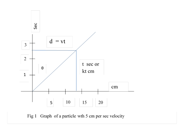
As velocity increases θ will increase; as maximum angle is 90 degrees and tan 90 is infinity, we think maximum velocity is without bounds.
Image 3
Two persons are sitting side by side. One may imagine vast spaces of Himalayan range; other may imagine vast spaces marina beach. The two spaces do not interfere with each other.
3. Some basic understanding.
3.1 One dimensional motion with uniform velocity is only considered here; this is sufficient to understand the basic concepts of timebit theory.
3.2 Particle here refers to either electron or proton. When mass is defined later, it is generalised to general dynamic particle.
3.3 Fixed distance particles (FDP) is extensively used to clarify concepts. When distance between any two particles in a set, do not change with time , they are referred as fixed distance particles (FDP). Let B,C, D.... be fixed distance particles (FDP) of set B; the distances BC may be d1 , CD may be d2, BD may be d3. Between d1, d2, d3, vector geometry applies .
FDP are assumed to have identical scales. The distance between FDP measured by these scales are true distances.
FDP also have synchronised clocks. It means if a clock of a FDP reads time ‘t’ , the clocks of other FDP also read the same time. The time measured by these clocks are true time with respect to its set.
Similarly P,Q,R may be FDP of set P, using same identical scales synchronised clocks. Similarly U,V,W may be FDP of set U
Particles of set B and set P and set U can have mutual velocity (ie) their distances change with time.
3.3.1 Let B and C are FDP; if B observes C at distance d at all times , then C would observe B at the same distance d at all times. This may be taken as operational definition of FDP. This idea is used to synchronise particles of the set.
3.3.2 If particles, B and P have mutual velocity, then if B finds P approaching then P would find B approaching ; similarly if B finds P receding then P would find B receding. This idea is used to prove existence of max velocity.
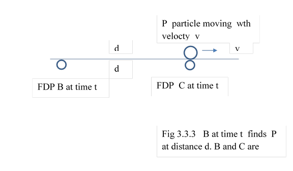
3.3.3 Let P moves with velocity v with respect to B ; at time t , B observes the position of P at distance d. This means, if there exists FDP C of set B, at distance d from B, C at time t would observe P at zero distance.
Further C at time would observe state of particle P, say its state of decay or time shown by P
3.3.4 Let P move with velocity v with respect to B At some moment, if B observes P at zero distance then P would observes B at zero distance; for both B and P, it is a common moment. This common moment can be used to initialise clocks of B and P.
3.3.5 Let B and C are FDP with distance d between them. Let particle P move with velocity with respect to B. At some moment if B observe P at distance d1, then C at the same moment would observe P at .distance (d1 +d) or ( d1-d ).
3.3.6 If B finds the velocity of P as v then all the FDP particles of B say C, D..would find the velocity of P as v. This common day experience is used to formulate Principle 3 of this thesis.
3.4 We understand line is one dimensional space or 1-D space.
Plane is two dimensional space or 2-D space. Lines can be drawn in all directions in a plane. Each line can be 1-D space. Also parallel lines, can be drawn with distance λ between them. λ is in the direction of second dimension .
Our world is 3-D space. Planes can exist in all orientations in this world. Each plane is a 2-D space. λ distance can exist between parallel planes. This λ distance is in the direction of 3rd dimension. The 3-D space is referred as ‘normal world ‘.
In timebit theory, 4-D space exists. 3-D spaces can exist in it, in all orientations. λ distance may exist between two parallel 3-D spaces. This λ distance is in the direction of 4th dimension. 4-D space is referred as ‘ total world ‘
3.5 Time : Generally it is thought, there is common flowing time , from past to future, in which events occur at every moment .
In this theory a person, through his memory, remembers past events in their sequence and also observes events of present moment. Memory by its sequencing, creates time as past, present and future. There may not be any general, common flowing time, but only personal time through memory
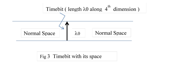
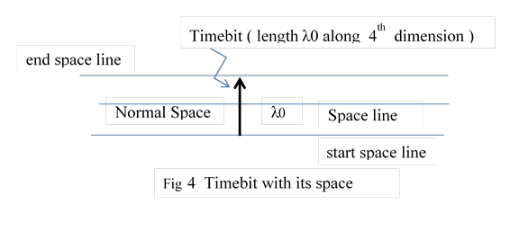
4 Timebit
4.1 Timebit Definition
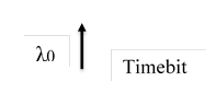
a ) Timebit is a tiny length λ0
b ) This λ0 is oriented to the fourth dimension of space which is not normally observable. It is indicated by an arrow.
c ) Perpendicular to it is, normal, linear, one dimensional space of infinite length. Visually it would look like fig 3
d) ) Lines perpendicular to timebit within its normal space are named as space lines. They don’t exist . but measurements are taken along these lines. Fig 4
![]() 4.2
Particle Dfinition
4.2
Particle Dfinition
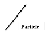
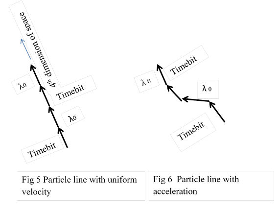
a ) The arrangement of timebits, end to end, in an infinite line, in the fourth dimension, is a particle.This line refered as particle line. If name of the particle is B, then it is B line.
b ) The line can be straight or curved, according to unifrom velocity or accelerated motion Fig 5, Fig 6
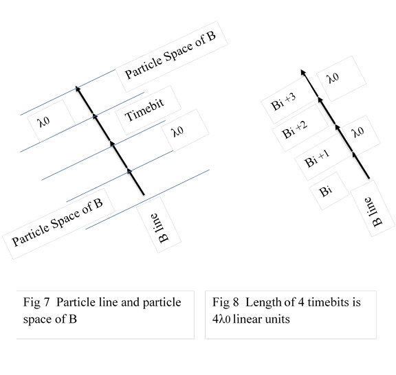
c ) The spaces of timebits in the particle line is called particle space. If the name of particle is B then it is referred as B Space Fig 7
d ) In a particle line, timebits can be numbered sequentially keeping an arbitrary timebit as number one. Numbering is done in the direction of arrow. Name of the timebit can be referred by the number it is assigned to, If ’i ‘ is the number of the timebit of particle B, then it is referred as Bi ; next timbit is referred Bi+1.Part length of the particle of n timebits is nλ0 linear units. Fig 8.
When context is clear , we simply refer them as i, (i+1), (i+2).
5 Observation Principle
5.1 In normal world, particles B ,P, U are presented as points. They may have different velocities. B at time t may observe P at distance d1; this is true distance with respect to set B. U at time t may observe point P at d2. It is true distances with respect to set U. . (3.3.3)
The same should be true for total world.
5.2 Principle 1
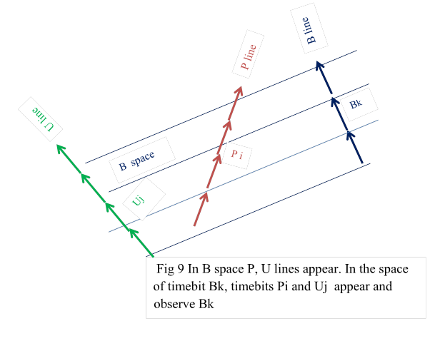
a ) In total world, in the space of a particle line B , other particle lines of P,U … appear. Fig 9
b ) Broadly, timebits Pi , Uj occur in some timebit space Bk and observe Bk Fig 9
c) Precisely, for mathematical amenability the following convention is followed.
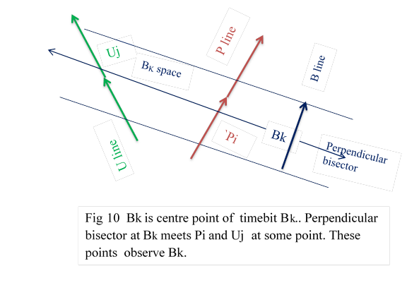
Centre point of timebit Bk is the observed point. It is also referred as Bk . Let the perpendicular bisector at Bk meet Pi and Uj at some points which may also be called of Pi and Uj . These points Pi and Uj observe centre point Bk at true distances that is , as in normal world. (3.3.3)Fig 10
d) As length of timebit is very small, name of the timebit, say Bk ,can be taken to refer some point in Bk
`
``
6 Orientation
6.1 In normal world, orientation refers to , up or down, left or right, front or back with respect to us. We fix it with reference to our FDP.
In total world, FDP lines and spaces maintain the same orientation as in normal world.
Each particle space is different and personal and exclusive. They do not interfere with other particle spaces.
So each particle line separately exists in other particle spaces
7 Time
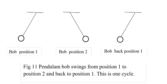
7.1 In normal world, objects occupy different positions at different times. We get the idea of time, from dfference between memory of previous positions of objects and present positions. Some objects change their positions repettively like simple pendulam from which we derive duration of time and continuity of time.
Fig 11 shows positions
pendulam bob that repeat itself. In all three positions bob is at rest and
changes its direction. Swing from 1 to 2 , back from 2 to 1 may be called a
cycle. We arbiirarily fix the duration of one cycle as one second. We
initialise, start of one cycle as one and count number of cycles for time elapsed.![]()
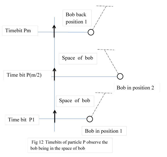
7.2 In total world, let some timebit of particle P, be fixed as P1..Let it observe the bob , at position 1, being in the space of bob. P(m/2), up by m/2 timebits, will observe the bob at position 2. Pm will observe the bob back at position 1 This is one cycle..Fig 12 .
P by its memory arbitrarily fixes this cyle as one second.
Let P1 is the start of this time zero and Pm is end of time, one second. Between P1 and Pm, one second time has elapsed. P2m will observe time as two seconds and P3m as three second.Thus duration and initialisation of time or reckoning of time, can be fixed by P, by its memory.
7.2.1 Direction of arrow is in the direction of increasing memory.
``
7.3 Each timebit is moment in time.There is no duration in a timebit. Its space is a still picture of other timebits of other particles. Between adjacent time bits there is duration of time which is refered as τ0. Between P1 and Pm there are m timebits and (m-1) durarions τ0 of time. The number m very large (m-1) can be approximated as m. So there are m timebits and m durations (τ0 ) of time.
8 Special feature 1
8.1 There is duration between two timebits and also distance between them.
If duration is one second between some two timebits, then the distance between them is referred as Ʋ . This Ʋ is , per second distance. It is refered as Ʋ linear units per second.
Later, we prove this Ʋ is the final maximum velocity..
8.2 If time difference between timebits is t seconds then distance between them is Ʋt linear units.
More generally, let Bt1 and Btn be first and nth timebit ; then length between Bt1 and Btn would be
n λ0 = l linear units.
l / t = n λ0 / t = Ʋ
or n λ0 / Ʋ = t sec
if n is one λ0 / Ʋ = τ0 sec
or λ0 / τ0 = Ʋ linear units per sec
This is a fundamental result which is true for both staight and curved particle lines.

8.3 So the least quantum of time is the duration between adjacent timebits τ0 which is λ0 / Ʋ. It is very small time; first because λ0 is small second because Ʋ very large..
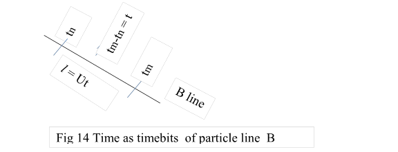
8.4 We can refer the timebit in a particle line B, as the time it refers to. Btm refers to timebit which reads its time as tm; Btn refers to timebit whch reads time as tn. If time difference Btn and Btm is tn-tm = t then length beween these timebits is Ʋ t.
It is simpler to refer Btn as tn and Btm as tm when context is clear.
When different particle is involved we use dashes. Btj can be referred tj ; Btk can be referred tk (without dashes)
Similarly Ptg can be referred as t’g and Uth can be referred as th”
8.5 We can draw particle lines continuously as timebits are very small. A timebit of a particle can be taken as a point in its particle line. This point reads an unique time as per its initialisation. So the point can be refered by the time reads.Fig 14
In particle line B, tm is the timebit that reads time tm. tn is the timebit that reads time tn. Time difference between these timebits is (tm-tn) = t sec. Length between them is Ʋt linear units.
9 Special feature 2
9.1 There is angle between particle lines B and P
9.2 In normal world P has velocity v with respect to B. Let B at tm find distance of P as d1 and at tn as d2.
If d2 – d1 = d and tn – tm = t Then d / t = v
Thus B finds the velocity of P as v. There is no angle involved.
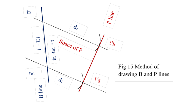
9.3 In total world the same data are drawn as shown in fig 15
We draw B line arbtrarily and mark some point as tm. Ʋt distance away we mark tn; tm and tn are the observing points of B. With tm as centre and d1 as radius we draw an arc. With tn as centre d2 as radius we draw another arc. The common tangent of these two arcs is P line. The tangents points t’g and t’h are observed points of P. This construction satisfies our definitions and Principle 1
The peculiarity of this construction needs to be discussed in few ways which will be done at later parts. The peculiarity is for one dimensional motion two distance measurements are required to fix one position. Uncertainity Principle directly stems from this consruction method’
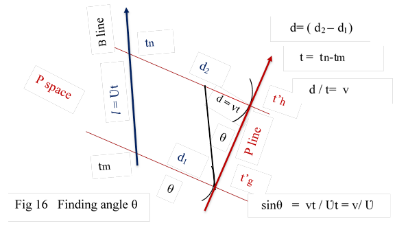
9.4 Now we have to find angle θ . Through t’g we draw a line parallel to B line. It meets space line from t’h at some point. From fig 16 we find
( d2 - d1 ) = d = vt from fig 16
sin θ = d / Ʋt = vt / Ʋt = v / Ʋ
or v = Ʋ sin θ
( In normal world we got a graph v = k tan θ . refer fig 1)
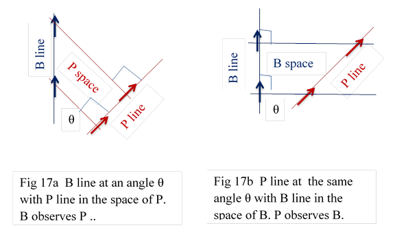
9.5 We have found angle between B and P lines in the space of P. The angle between B and P line in the space of B is same. We will state this as Principle 2
10 Principle 2
If the angle between B and P lines in the space of P is θ, then in the space of B it would be same θ. Fig 17
````
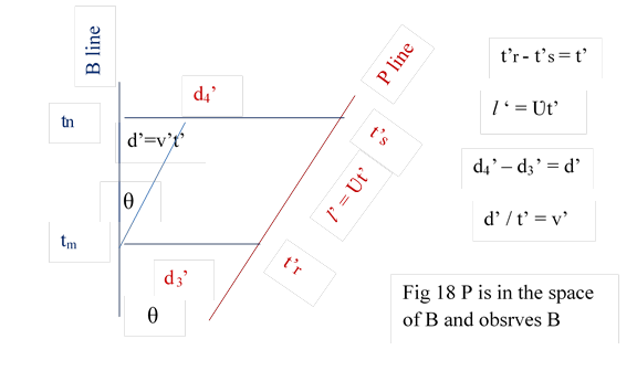
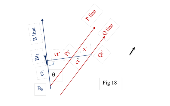
10.1 Lemma : If the velocity of P with respect to B is v, then the velocity of B with respect to P is same v.
In the space of P, angle between B and P is as per fig 16:
sin θ = v / Ʋ
In fig 18 P line is in the space of B. Angle is kept θ as per principle 2
sin θ = v’t ‘/ Ʋ t’ = v’/ Ʋ
As θ and Ʋ are same , v = v’
10.2 Maximum angle of θ = 90◦
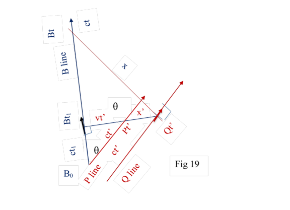
10.2.1 There is a max angle of θ = 90 ◦ between particle lines.The proof is somewhat heuristic. We use the sense stated in 3.3.2
10.2.2 In fig 19a B line is in the space of P; so B observes P. There is an angle θ< 90◦ between B and P lines. tm obsrerves t’p at distance d1. tn observes t’q at distance d2. d2 is greater than d1. So B observes P receding.
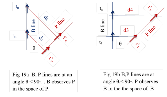 In
fig 19b P line is in the space of B; so P observes B There is an
angle θ◦< 90◦ between B and P line. t’t
observes tr at distance.d3. t’u observes
ts at distance d4. d4 is greater than d3.
So P also finds B receding.
In
fig 19b P line is in the space of B; so P observes B There is an
angle θ◦< 90◦ between B and P line. t’t
observes tr at distance.d3. t’u observes
ts at distance d4. d4 is greater than d3.
So P also finds B receding.
This is as in normal world. (3.3.2)
10.2.3 In fig 20a angle between B and P is more than 90 degrees.
In 20a particle line B is in the space of P and observes P. tm observes t’p at distance d1. tn observes t’q at distance d2. d2 is less than d1. So B finds P approaching.
`````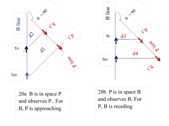
In fig 20b particle line P is in the space of B and observes B. t’p observes tn at distance d3. t’q observes tm at distance d4. d4 is greater than d3. So P finds B receding.
In the first case B finds P approching and in the second case P finds finds B receding.
This is not so in normal world. So angle θ more than 90 degrees, between paticle lines is not possible.
10.2 Maximum angle between particle lines is 90 degrees.
11. Maximum velocity.
11.1 We have already found in 9.4 , if the angle between particle line is θ, then sin θ = v/Ʋ, where v is mutual velocity of particles and Ʋ is length of paticle line between points whose time difference is one second.
sin θ = v/Ʋ
maximum angle as per 10.2 is 90 degrees.
sin 90 = 1 = v/Ʋ
Maximum velocity v = Ʋ
So maximum velocity exists as stated in the first paragraph of this thesis.
12 Velocity of light.
12.1 In normal world ,velocity of light ‘ c’ is maximum. We can equate
Ʋ = c
We can say, Ʋ is experimentally found to be ‘ c ‘; no principle is required.
Kinetic theory of gases predicts, there exists is a minimum temperature; experimentally it is found as -273 degrees.
Similarly timebit theory predicts, there exists maximum velocity; experimentally it is found to be ‘c ‘.
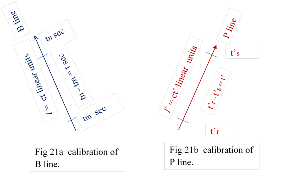
13 Calibration of particle line.
In fig 13 , we had conceptualy calibrated particle line, as Ʋ linear units as one second. We have found Ʋ = c We, now can actualy calibrate the paticle line as ‘ c’ linear units as one second. c = 3 x 10⁸ meters per second. fig 21.
13.1 “If time difference between two points on a patrticle line is t then distance between them is ct “
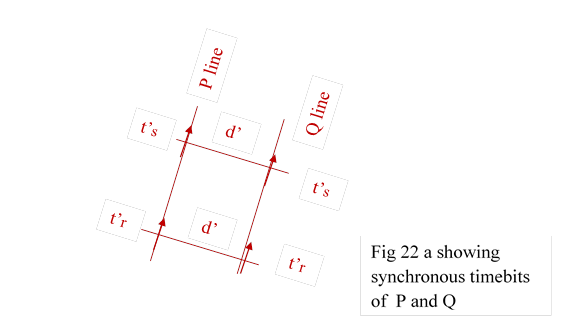
14 Synchronous particles and synchronous timebits. Definition
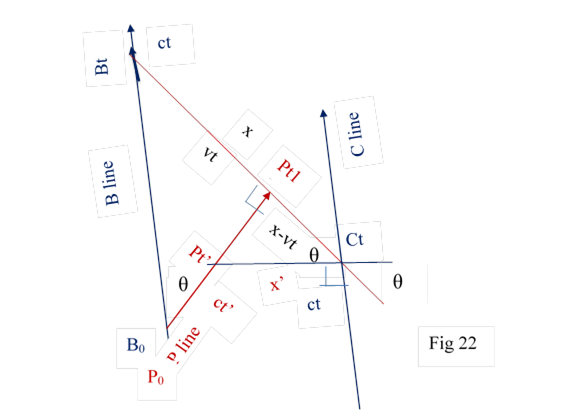
14.1 In normal world fixed distance particles (FDP) are named as synchronous paticles. Particles B,C,D are in FDP of set B and have synchronised clocks. B at time t would observe C,D to read the same time t, hence the name.
14.2 In total world FDP particles are parallel lines Fig 22 because their distances are constant.
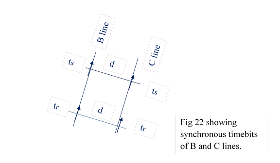
Timebit tr of B observe a timebit of C which would read time same tr because clocks are synchronised.Distance between B and C lines is d asin normal world
Timebit tr of B line and timebit tr of C line are named as synchronous timebits. Similarly ts of B and ts of C are sinchronous timebits.
Similarly t’s of P line and t’r of Q line are synchronous timebits.similarly t’s of P and t’s of Q are sinchronous timebits. distance between P and Q lines is d’ as in true world.
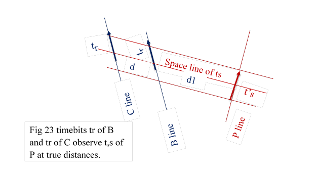
15 Principle 3
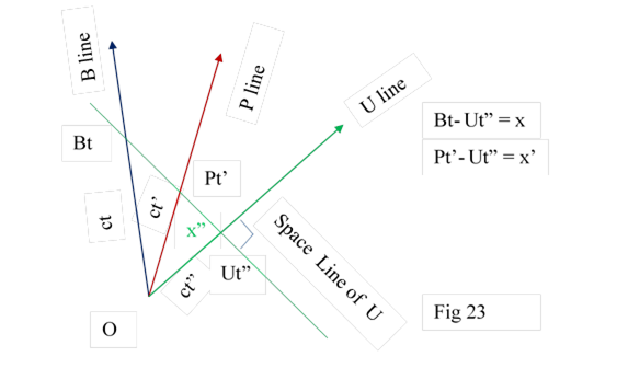
15.1 If timebit tr of particle B, observes timebit ts‘ of particle P, then tr is in the space of ts’. All the synchronous timebits of tr ( other FDP C,D..)appear in the same space ts’ in their true distances. Fig 23.
15.2 If d is the distance between FDP B and C in normal world then distance between timebits tr of B and tr of C would be d in total world also
15.3 If B at time tr observe ts’ of P at distance d1 in normal world then the distance beween tr of B and t’s of P would be same d1, in the total world. Also distance between B and C in the space of P would be the true distace d.
15.4 B and C lines are in either side of P line. Timebits tr of B and tr of C are in the space of t’s of P at distances d1 and d2,
d = d1+d2. All three
distances are true distance as per 3.3.3 `````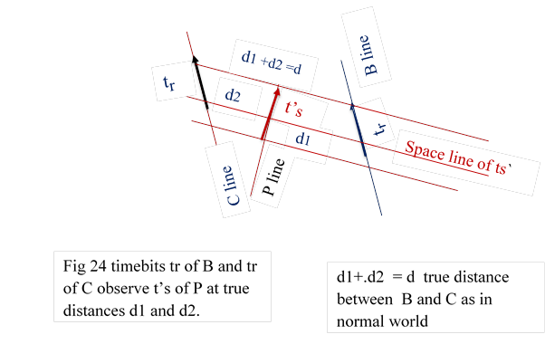
Conclusion
We have defined timebit as tiny length λ0, represented by an arrow... Perpendicular to it, is the normal one dimesional space. Arrangement of timebits with their spaces in a line is defined as particle. Such a line is referred as particle line and spaces of timebits in the particle line, is referred as particle space. In the space of particle line other particle lines appear . Thus particle space is the still picture other particle lines Their timebits observe the timebit providng space
Time is indicated by the change in memory of timebits ( if they have one). Direction of arrow is indicated by direction of increasing memory
With these ideas we have found maximum velocity exists and we have equated it to velocity ‘c’.
In part 2 we will derive all the results of relativity and also suggest crucial experiment to validate timebit theory.
Appendix A of Part one
Suppose The velocity approaches c and becomes c , then adopting the procedure 9.3 we would find the entire particle line is in the space of single timebit of observed particle line.
The above fig shows B observing P which has the velocity c. Entire particle line of B is in the space of timebit k of P observe k .This means m of B is observes k of P at zero distance and, m+1 observes the same k at λ0 distance and m+2 observes at 2 λ0 distance so on. So all timebits of B observess same timebit (phase ) of P, As λ0 /τ0. = c we find this phase moves with velocity c,
Timebit Theory Part 2
( Kinematic relationships)
By
S.Nagarajan ME (Str)
Timebit Theory Part 2
( Kinematic relationships )
1 Recapitulation
In the first part we have extensively used ‘fixed distance particles’ (FDP) to clarify distance and time measurements. Three definitions were made:
Dfinition1 Timbit and its space
Definition 2 Particle, particle lines and particle spaces
Definition 3 Synchronous timebits
Three principles were enunciated.
Principle 1 observation
Principle 2 Angle between particle lines.
Principle 3 Synchronous timbits observation.
We also established if two particles have mutual velocity v in normal world, then in total world their particle lines will have angle θ between them where sin θ = v/c .
What we mean by observation was stated in 3.3.3 of first part whch is repeated here; It is true for normal world and total world.
“ Let P moves with velocity v with respect to B ; at time t , B observes the position of P at distance d. This means, if there exists FDP C of set B, at distance d from B, C would observe P at zero distance at time t.”
Another point 13.1 of part one is repeated here:
“A timebit in particle line B (say) can be arbitrarily initialised that it reads its time as zero; it is referred as B0 .Few timebits later, a timebit may read the time as t; this timebit is called Bt. The distance between Bt and B0 is ct..
This is true only for total world.
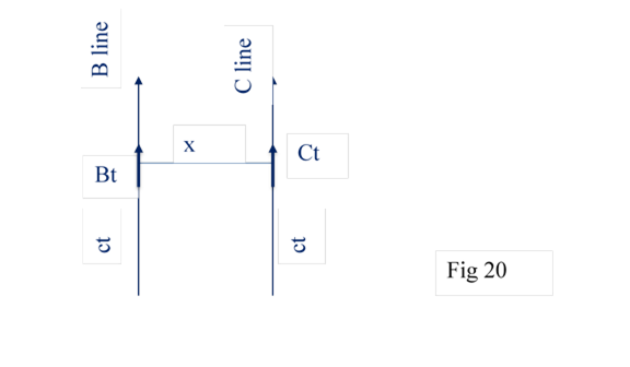
2 Observation
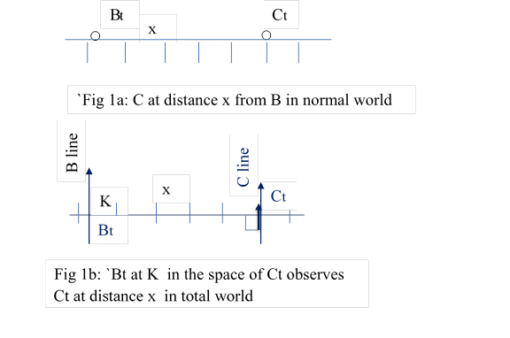
2.1 Two FDP particles B and C are at distance x ; at time t , let Bt observe Ct; their pictures in normal world and total world are shown in fig1. K the is point in the space of Ct from which Bt observes Ct.
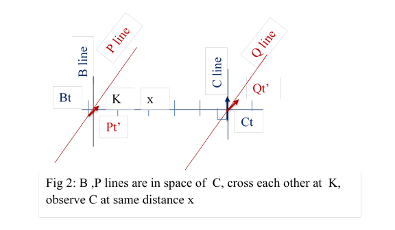
2.2 Let Pt’’ of some other particle line P with velocities v pass through K. Pt’ will also observes Ct at same distance x, as per principle one and 3.3.3 of part one. Fig 2. Also FDP points of B and P at any particular distance , exactly coincide with each other
This means if there is a FDP line, Q at distance x from P, its timebit Qt’ will cross the timebit Ct and read its time as t. and it would be at zero distance with Ct. By the information of Qt’ only, Pt’ understands, it observes C at distance x and its time is t.
2.3: B, P lines cross each other at K. But they will not observe each other because they are not in the space of each other.
It looks like, B and P observe C in separate layers or spaces.
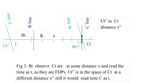
2.4 Suppose some particle Ut” is in the space Ct at L, it will observe Ct at some distance x” ; also Ut’’ would read time of C as t. It means if there exists Wt”, FDP of U at distance x”. it would be at zero distance from Ct and it will also read the time of C as t. Fig 3
This is as per 3.3.3 and principle one
2.5 Finally the distance and time of measurement are true ones in the sense 3.3.3 of part 1
3 Velocity observation
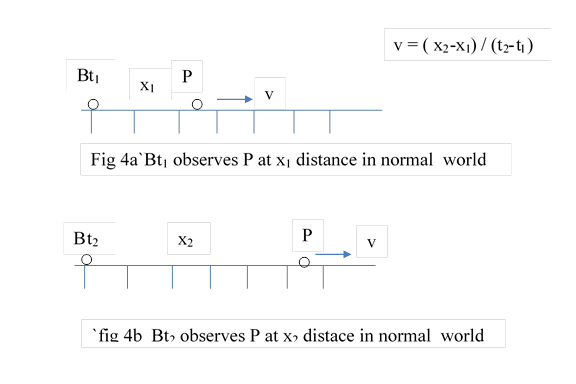
3.1 In normal world let particles B and P have mutual velocity v ; let Bt1 observe P at distance x1. Bt2 observe P at a distance x2 . Velocity v =( x2 – x1) / (t2- t1) .
We can visualise a scale as FDP points of B with synchronised clocks at all distances. At zero of the scale particle B exists. P is moving along the scale, Bt1 observes P at distance x1 along the scale. Bt2 observes P at distance x2 (fig 4) .
We have to draw two different true pictures to show the positions of particles B and P, one at time t1 and other at time t2 (fig4). Both pictures can not be combined into one pictures. Graph shown in fig1 of part one, is the best thing we can do, which is not a true picture.
`
3.2 In total world we get the same result; but its description is very different. Detailed procedure of finding v is given in part one.
Particle line B must be in the space of P to observe P . Particle lines B and P are at an angle θ defined by sin θ = v/c . B line is in the space of P as shown in fig5.
Particle lines are calibrated such that if time difference is t then the distance between them is ct. (13.1 of Part One)
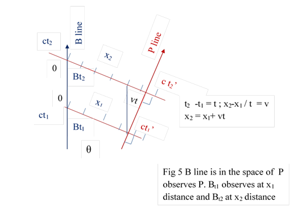
In P space particle line of B appear and observe P as per principle1. Bt1 observe Pt1’ at distance x1. Bt2 observes Pt2’ at x2. The velocity is (x2-x1)/ (t2- t1) = v. If t2-t1 = t then (x2-x1)/t = v and x2 = x1+vt
There is a possible doubt that FDP of P at time t1’ , at distance -x1 can observe t1 of B. This is not so because P is not in the space of of B.
So timebits of particles appearing in the timbit space of Pt’ can observe only Pt’; they cannot observe each other.
3.3 Fig 6. Similarly Pt1’ observes Bt1 at distance x1’. Then Pt2’ observes Bt2 at distance x2’. In both instances P is in the space of B. If ( t2’-t1’) = t’ then v’ = v = ( x2’-x1’) / t’ ; x2’ = x1’ + vt’
``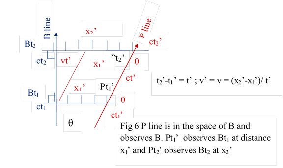
It is one of the paradoxe,s to observe one position another particle, we have to make two measurements; or we have to know its velocity
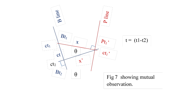
4 Reciprocal observation
4.1 In normal world we think, particles B, P as points, in a general common space. We say, particle B, at time t, observe particle P at a distance x. In pre relativity physics, observed time of P would be same t. At time t, P also finds B at distance x.
4.2 In total world, timebit theory finds above statements are true only for fixed distance particles (FDP ).
4.3 B and P have mutual velocity v, receding from each other. Bt1 observes Pt1’ at a distance x, and reads its time as t1’.Fig 7
If Pt1’ observes, some point , Bt2, at distance x’, and reads its time as t2,
What are x’ and t2 ?
The above question is asked by B as it only has necessary data. Pt1’ is first observed then it observes.
4.4 In fig 7 Bt1 is in the space of Pt1’ and observes Pt1’ at distance x. Let Pt1’ in the space of Bt2 and observes Bt2 at distance x’.
From fig 7 x’ = x cos θ = x (1-v2/c2)1/2
As t2 < t1 c(t1-t2) = ct =x sin θ = xv/c
( t1- t2 ) = t = xv/c2 ( earlier )
t2 = ( t1- xv/c2 )
So B deduces Pt1’ would observe it
at distance x’ = x (1-v2/c2)1/2
and reads the time of B as = t2 = ( t1- xv/c2 )
4.5 There another related question. Let Bt1 observe Pt1’ at x distance and find its time as t1’, as before, Let Pt2’ observe Bt1 at time t2’ at distance x’ .
We know x, t1, t1’ . What are t2’ and x’ ? (Fig 8)
B again asks this question as it has the necessary data. Here Bt1 first observes then gets observed.
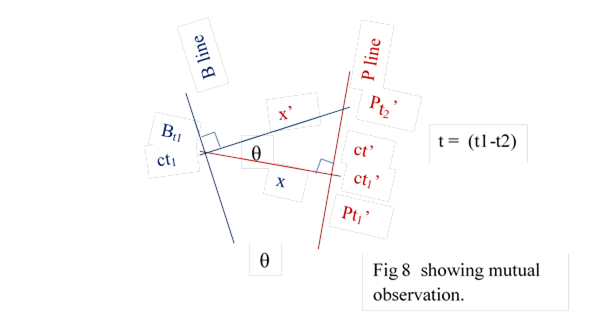
From fig 8 x’ = x / cos θ = x / (1-v2/c2)1/2
c(t2’-t1’) = ct’ = x tan θ
Dividing by c (t2’-t1’) = t’ = x tan θ / c
t2’ = t1’ + x tan θ / c
Where tan θ = sin θ / cos θ = ( v/c) /(1-v2/c2)1/2
5 Time dialation
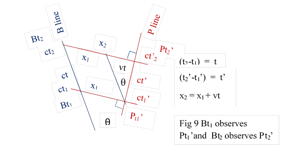
5.1 Let Bt1 observe Pt1’ and again Bt2 observe Pt2’ Observing duration of B is (t2-t1) = t. Observed duration P is ( t2’-t1’) = t’. What is the relationship between t and t’ ?
Now we are familiar with fig 9 that shows all the data of the problem. B line is in the space of P and observes P. From fig 9 Bt1 observes Pt1’ at distance x1 and Bt2 observes Pt2’ at distance x2.
(t2-t1) = t. and (t2’-t1’) = t’.and ( x2-x1) = x
c2t2 = c2t’2 + v2t2
dividing by c2 and transferring
t’2 = t2 (1-v2/c2)
t’ = t ( 1- v2/c2 )1/2
As v < c t’ < t
We think P takes a longer time to become t ; hence the name time dilation. This phenomena is entirely due to Principle 1.
7 Length contraction
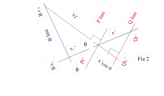
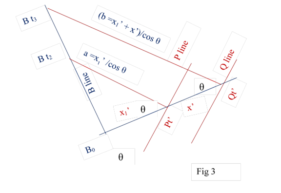
7.1 Let P and Q are FDP with true distance x’. They move at velocity v with respect to B.
If B observes the distance between P and Q as x, how x and x’ are realated ?
. 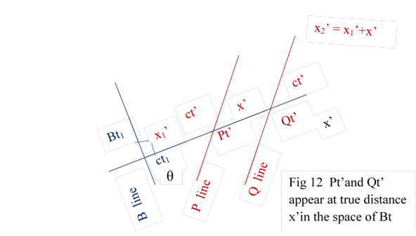 7.2.
P and Q are FDP and distance between them is x’ which is defined as true
distance. Principle 3 states synchronous timebits of Pt’ and Qt’ appear in the
same timebit space of Bt1 at true distance x’ and observe Bt1
Fig 12
7.2.
P and Q are FDP and distance between them is x’ which is defined as true
distance. Principle 3 states synchronous timebits of Pt’ and Qt’ appear in the
same timebit space of Bt1 at true distance x’ and observe Bt1
Fig 12
So Pt’ and Qt’ appear in the space of Bt1 and observe Bt1 at distances x1’ and x2’ = (x1’+ x’). Fig 12
Let Bt1 observe Pt2’ at distance x1 and Qt3’ at distance x2 .It may be noted observing time is same t1 for both cases. It would conclude distance between P and Q is( x2- x1) = x ( fig 13)
By reciprocal observation
x1 = x1’ cos θ fig 13
x2 = x2’ cos θ = (x1’+x’) cos θ
x = (x2 - x1) = (x1’+x’) cos θ - x1’ cos θ
= x’ cos θ = x’( 1- v2/c2 )1/2
x = x’ ( 1- v2/c2 )1/2
as v < c x < x’
So observed distance x is less than true distance x’
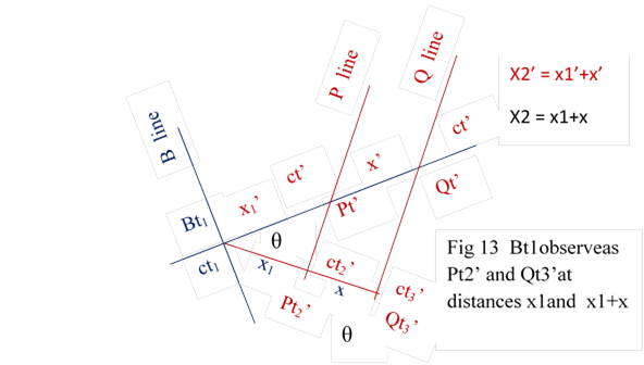
. This is known as length contraction. This happens because of change of space and Qt3’ is observed earlier than Pt21’.
8 Lorentz Transformation.
8.1 We have so far derived our results with arbitrary initialisation (ie) without any reference to each other. Now we will link the initialisations.
The problem can be stated as follows:
If B and P are two FDP systems with mutual velocity v, then how the FDP of one system are related to the FDP of other, with respect to distance and time?
8.2 We will take two
particles B and P that have mutual velocity v. B0 and P0
are at zero distance to each other. B0 and P0 are
initialised as time zero. Angle between them is θ, defined by sinθ =
v / c. Fig 14. Distance between B0 and Bt is ct; distance between P0
and Pt’ is ct’. 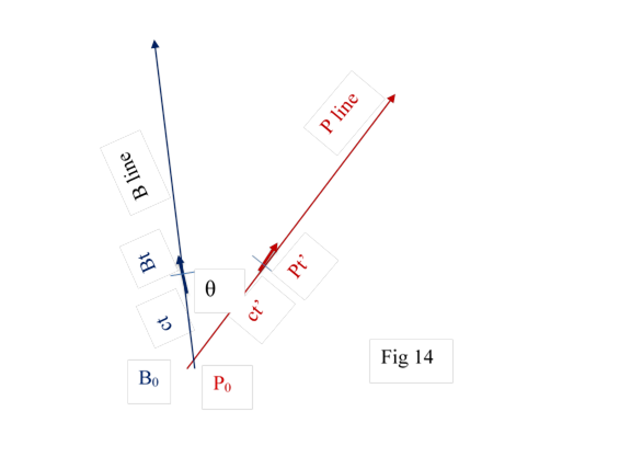
Let some Bt
observe Pt’ at x1 distance, being in the
space of Pt’. At zero time B observe P at zero distance (Fig 15); at t time B
observes P at vt distance Fig 15. Also Bt reads the time of P as t’.
(3.3.3) of part one.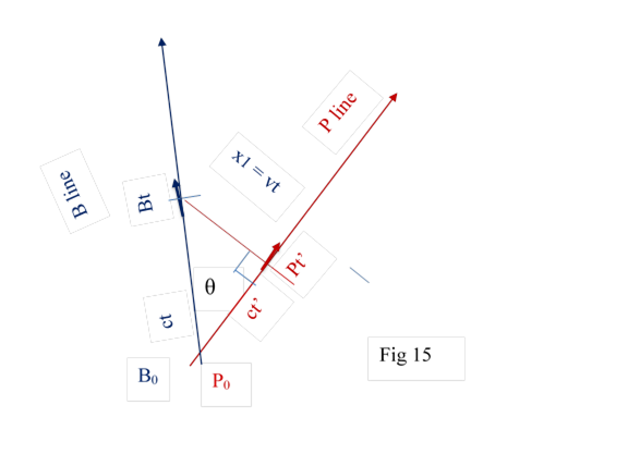
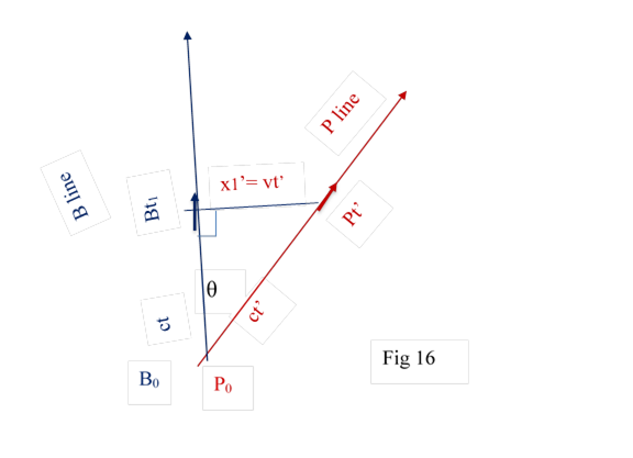
Similarly Pt’ would observe some Bt1 at diatace x1’’= vt’ Fig 16 Also Pt’ would observe time of B as t1.( 3.3.3 of part one)
````
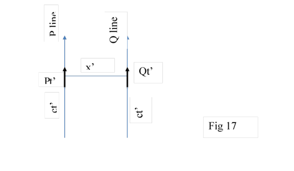
8.3 P and Q are FDP with distance x’ between them , Pt’ at any time t’ would observe Qt’ at time t’ at a fixed distance at x’.(vice versa).Fig 17
8.4 Let P line and Q line appear in the space of some B. Some Pt’ would observe Bt at distance vt’. Qt’ would observe Bt1 at distance (x’ + vt’ ) Fig 18. Principle 3 Fig 18
By reciprocal observation Bt would observe Qt’ at distance x; from fig 19
x = ( x’ + vt’) / cos θ = ( x’ + vt’) / ( 1- v2/c2 )1/2
and
ct = ct’ cos θ + (x’ + vt’ ) tan θ
ct = ( ct’ cos2 θ + (x’ + vt’ ) sin θ ) / cos θ
Dividing by c
t = ( t’ ( 1- v2/c2) + (x’ + vt’ ) v/c2 ) / cos θ
cancelling t’v/c2
t = ( t’ + x’v / c2 ) / cos θ = (t’ + x’v / c2 ) / ( 1- v2/c2)1/2
So B would observe Qt’ at distance x and time t where
x = ( x’ + vt’) / cos θ = ( x’ + vt’) / ( 1- v2/c2 )1/2
t = ( t’ + x’v / c2 ) / cos θ = (t’ + x’v / c2 ) / ( 1- v2/c2)1/2
The above equations are called Lorentz transformation which transforms the FDP coordinates of P system into coordinates of B system.
``
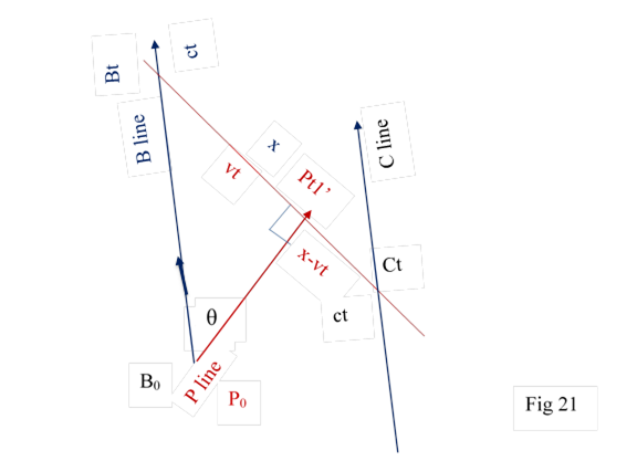
8.4 Similarly B and C are FDP with distance x between them , Bt at any time t would observe Ct at time t at a fixed distance at x.Fig 20
Let B line and C line appear in the space of Pt1’. Distance between Bt and Ct is x as per principle 3. Bt would observe Pt1’ at distace vt as per initialisation. In the space of Pt1’ distance between Pt1’ and Ct is (x – vt). Fig 21 (ie) Ct would observe Pt1 at distance (x-vt).Fig 21
8.5 If we draw a perpendicular to C line at Ct , it would meet P line at Pt’. From Fig 22 Pt’ observes Ct at distance Fig 22
x’ =( x-vt) / cos θ = x’ = ( x-vt) / ( 1- v2/c2 )1/2
ct’ = ct cos θ - ( x-vt) tan θ
=( ct cos2 θ - ( x-vt) sin θ) / cos θ
= ( ct ( 1-v2/ c2 ) - ( x-vt) ( v/c) ) / cos θ
t ‘ = ( t - v x / c2 ) / cos θ
= ( t - v x / c2 ) / ( 1- v2/c2 )1/2
So P would observe C at distance x’ and time t’ where
x’ = ( x-vt) / ( 1- v2/c2 )1/2
t’ = ( t - v x / c2 ) / ( 1- v2/c2 )1/2
This is the second set of Lorentz transformations which trasforms FDP points of B system into P system.
-
9 Invariance
9.1 Length and duration in a FDP system, say of B, do not change when measured from any FDP. When a scale or clock moves with velocity v, their length or duration should not change, as believed in pre relativity physics for variety of sound reasons. They were invariants.
9.2 We now know observed length is less and clock is observed to run slower. Now is there an invariant quantity? We have proved length is contracted because we see earlier position of farther end and clocks run slower because we see earlier position of clock. Both phenomenon is due to Principle one.
9.3 If L is true length or FDP length, and it moves with velocity v with respect to B then contracted length is:
l = L cos θ
or L = l / cos θ is invariant for any observer
9.4 Similarly if for FDP true duration is T the observed duration with respect to B is t:
t = T cos θ
or T = t/ cos θ is invariant for any observer.
9.5 In Fig 23 B, P, U particle lines are drawn with common initialisation point O.Bt and Pt’ observe Ut” being in its space line. from fig 23
(ct)2 - x2 = (ct”)2 = ( ct’)2 – x’2
ct”2 is invariant which is the distance between origin and Ut”
10 Transformation Velocity
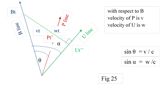
10.1 Let B, P, U be different FDP systems. B observes velocity of P as v and U as w. P will observe velocity of B as v and U will find velocity of B as w, as they are mutual velocities. We have to find the velocity of U with respect to P.
10.2 For simplicity let
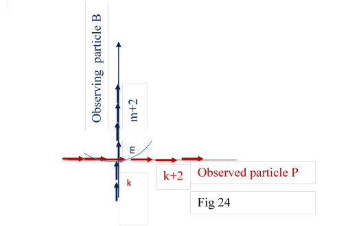
B,P, U particle lines meet at a point as shown in fig 24. Let them be
initialised as zero time at this common point.
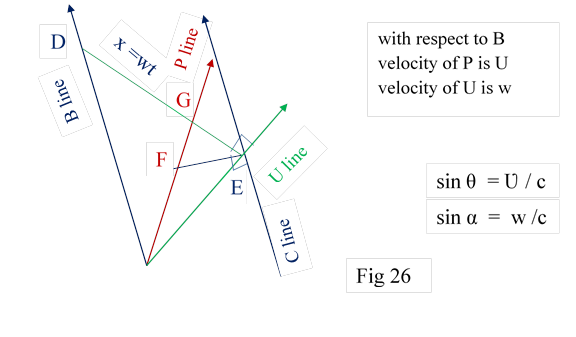
Let B at time t observe U; as velocity of U is w , B observes it at distance x = wt . Fig25 It means there is a FDP point of B at distance x which is observed by P at distance x’ and time t’( F of fig 26).By Lorentz transformation :
x’ = (x-vt) / cosθ ; t’ = ( t – vx/ c2) / cosθ
x is the position of FDP of B which observes U at zero distnace
Now P does not observe U, but FDP of B for which Lorentz transformation applies. It is assumed this gives velocity w’of U with respect to P
w’ = x’ / t’ = ( (x-vt) / cosθ ) / (( t – vx/ c2) / cosθ )
= (x-vt) / ( t – vx/ c2 )
Dividing by t = ( x/t – v ) / 1 – v (x/t) / c2
As x/t =w we get
w’ = ( w-v) / (1-vw/ c2 )
10.2 The problem is, it gives rise to some inconsistency. In fig 26 Point D on B line observes E of U line, along DE line as DE is perpendicular to U line. It means FDP line C of B at distance x = wt passes through E. E is on both C and U line. E on C is observed by F on P line. This gives us the expression w’ which is velocity of U with respect to P. If P actually observes U, it must be along DE at G or at some point, along the line parallel to DE. So we have two points on P line which observes point E. This inconsistency comes because,
1) P at F observe FDP of B , C at E which is at zero distance with U, in the space of C; fig 26
2) P at G observes directly U, at same E, in the space of U. fig 26
This leads to some uncertainty in the observation of distance and velocity which are likely to be solved at quantum levels.
11 Experimental Verification.
11.1 Do timebits exist for a particle ?
In normal world, let a particle move with uniform velocity in a circle of radius r. Let it execute n revolutions per second. One revolution will be executed in 1/ n second, Let another particle stay at rest. We think both have endured same quantum of time. Fig 27
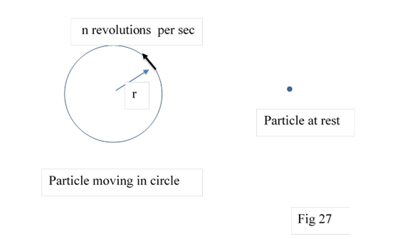
In timebit theory time elapsed depends number of timebits passed. In 1/n second, particle at rest would pass the distance c/n .
Particle moving in circle will be a helix with pitch c/n. Length of a helix for one pitch is ( fig 28 )
( (c/n )2 + (2πr)2 )1/2 = ( c/n) ( ( 1 + (2πrn/c )2 )1/2
= ( c/n) (1 + (1/2) (2πrn/c )2 ) = ( c/n) (1 +2π2 r2 n2 / c2 )
= c/n + 2π2 r2 n / c
One pitch length of particle at rest = c/n.
Length of helix per revolution is = c/n + 2π2 r2 n / c
Length for n revolution or one second = c + 2π2 r2 n2 / c
Length fot t seconds = ct + 2π2 r2 n2 t / c
Time endured by helix t seconds = t + 2π2 r2 n2 t / c2
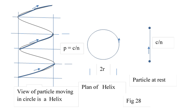
11.2 If we compare the clock at rest and clock moving in circles, the later will show more time by 2π2 r2 n2 t / c2 where n is number of revolutions per second and r is the radius of the circle and t is the time elapsed by the stationery clock.
While stationery decaying elements decay for time t , rotating elements will decay for time t + 2π2 r2 n2 t / c2
11.3 Suppose we assume n = 100 revolution per second, r = 10 m , t as one hour. Extra tme experienced
2π2 r2 n2 t / c2 = 2 (3.14)2 (100)2 (10)2 (3600) / (3)2(108)2
= 2 x 9.86 x 36 x 108 / 9 x 1016
=7.8 x10 -8
Time elapsed for element moving in circle is
3600 + 7.8x 10⁻⁸
Difference is a very small quantity which can be made larger by choosing larger n, r and t. If such an accuracy is possible the hypothesis of timebits can be verified’
11 Conclusion
We have assumed three new principles about particle and observation and derived all the results of relativity. An experiment that would decide distinctive feature of this theory has also been described. The chief feature is every particle creates its own space and time in which other particles of world exist .Also it has enough theoretical space that the theory can be expanded to quantum levels and general relativity.
In the next parts we will define mass and charge and electromagnetic waves and other aspects of physics. There is also a question why the world is three dimensional which we hope to address. Finally the present theses needs to be put in a more analytic and algebraic form.
Appendix A Part 2
Length Contraction : Alternate ways
1 Let P and Q be
FDP with true distance x’. They have velocity v with respect to B.
Let them observe B at sometime. By Principle 3 it would look like the
following Fig 1 where x1’ and x’ are true distances.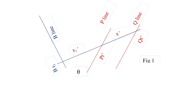
If we draw a perpendicular to P line at Pt’ it will meet B line at Bt2. Fig 2.
Bt2 would observe Pt’ at distance x1. If we again project the perpendicular to meet Q line, Bt2 would observe Qt’ at distance x1 + x’cosθ. Fig 2 Difference between the two measurement is
x1 + x’cosθ – x1 = x’cosθ = x’ (1-v2/c2 )1/2
2 There is a third more informative way of finding length contraction. Fig 3
Bt2 observes Pt’ at time t2 = ( x1 tan θ) / c
Bt3 observes Qt’ at time t3 = (( x1 +x’)tan θ) / c
Difference between t2 and t3 =
t3 – t2 = (( x1 +x’)tan θ) / c - ( x1 tan θ) / c = x’tan θ/ c
In this time position of Q has increased the distance from B
= (x’tan θ )v/ c
Distance Bt3 to Qt’ = (x1’+ x’) / cos θ
Distance when Qt’ is observed by Bt2 =
(x1’+ x’) / cos θ - (x’tan θ )v/ c
= (x1’+ x’) / cos θ –( (x’sin θ )v/ c) / cos θ x1’/ cos θ + x’(1 - v2/ c2) / cos θ (1)
Pt’ is observed by Bt2 at distance = x1’/ cos θ (2)
Subtracting 2 from 1 we get = x’(1 - v2/ c2) / cos θ
= x’(1 - v2/ c2)1/2
So contraction happens due to the farther end is observed earlier than near end.